Array data structure

Oct 17, 2024

—

1. Introduction

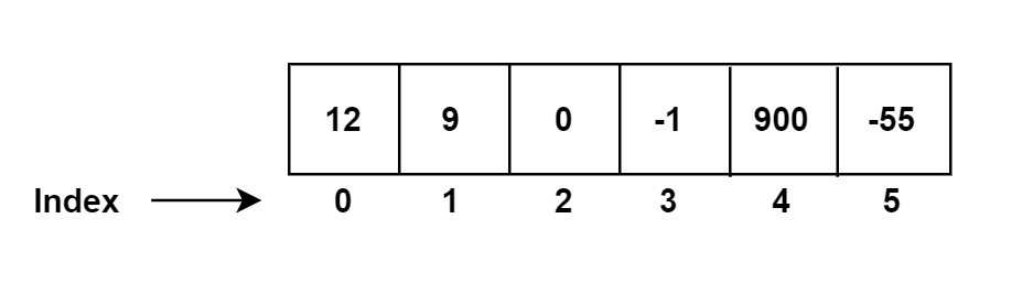
The goal of a data structure is to make operations as fast as possible such as inserting new items or removing given items from the data structure. Arrays are data structures where all the items are identified by an index – an integer starting with 0. The items of the array are located right next to each other in the main memory (RAM) and can be accessed by index. The reason why we can use indices is the fact that the items are located right next to each other in the memory.

The primary benefit of array data structures is their ability to support random indexing, allowing for extremely fast access to elements using their indices.

The index starts with zero (0). Every single item in an array can be identified with a given index. In Java, C and C++ we can store items of the same type in a given array. If we know the index of the item, we can get it extremely fast in the constant running time complexity O(1).

The main problem with arrays is that we need to know the number of items we want to store in advance.

2. Two dimensional array

A two-dimensional array can be thought of as an array of arrays. Each element in a 2D array is accessed using two indices: one for the row and one for the column.

This structure is particularly useful for representing matrices, tables, or images.

In Java, a two-dimensional array can be declared and initialized as follows:

// Declaration
int[][] array;

// Initialization
array = new int[3][4]; // A 3x4 array (3 rows and 4 columns)

// Or in one line
int[][] array = new int[3][4];

You can also initialize a 2D array with specific values:

int[][] array = {
    {1, 2, 3, 4},
    {5, 6, 7, 8},
    {9, 10, 11, 12}
};

You can access elements in a two-dimensional array using their row and column indices:

int value = array[1][2]; // Accesses the element in the second row, third column (value is 7)

3. Array Data structure applications

Array data structures are widely used in computer science due to their efficiency in organizing and managing data. Here are some key applications:

Arrays are used to represent matrices and perform matrix operations.
Arrays are the foundation of many sorting algorithms like: Bubble Sort, Merge Sort, Quick Sort.
Arrays act as buffers when transferring data between different parts of a program or between hardware and software components.
Arrays of registers are used in processors to store temporary data during computation.
2D and 3D arrays are used to store pixel values and other graphical elements.
Arrays are used to model grids, boards, and spatial structures in video games.
Arrays are crucial for storing intermediate results in dynamic programming solutions, which is essential for solving problems like: Fibonacci sequence, Knapsack problem, Longest common subsequence (LCS).
Arrays are often used as the underlying structure for more complex data types like: Stacks, Queues, Heaps, Hash tables.
Arrays are commonly used in search algorithms like: Binary search, Linear search.

4. Adding items

We can insert new items to the end of the array data structure until the data structure is not full. This operation has O(1) running time complexity.

4.1 What if the data structure is full?

If an array data structure is full, meaning it has reached its maximum capacity (based on its size), there are several potential issues and solutions depending on the type of array being used and the application. Here’s what happens and what can be done:

Static Arrays (Fixed-Size)

In a static array, the size is fixed when the array is created. Once the array is full, no new elements can be added without some form of resizing or reallocation.

Problems:

No more space for new elements: You can’t add any more data to the array because it is already at its defined capacity.
Out of bounds errors: If an attempt is made to access an index beyond the array’s size, it may result in an “index out of bounds” error in many programming languages.

Solutions:

Create a new larger array: Allocate a new array with a larger size, copy the existing elements into it, and then add new elements.
Dynamic Arrays (e.g., ArrayList in Java or List in Python): These structures handle resizing internally by automatically increasing their size when full. The underlying array is typically resized by creating a new array that is often double the size of the original, and copying the old data over.
Time Complexity: Resizing an array has a time complexity of O(n) because all the elements need to be copied into the new array.
Linked Lists: If frequent resizing is undesirable, a linked list or other data structures may be used, as they do not require continuous memory allocation.

Dynamic Arrays (e.g., ArrayList, Vector)

In dynamic arrays, which are implemented in higher-level languages, the array will automatically resize itself when full.

Problems:

Performance hit: When the array resizes, it requires creating a new array and copying all existing elements to it. This process can be expensive in terms of time.
Wasted memory: After resizing, dynamic arrays may have unused memory, leading to wasted space until the array fills up again.

Solutions:

Optimize resizing strategy: Use strategies like geometric growth (doubling the size of the array) to minimize the number of times resizing happens.
Preallocate memory: If the approximate size of the array is known in advance, you can preallocate memory to avoid frequent resizing.

Circular Buffer/Array

A circular array (used in fixed-size queues) overwrites the oldest data once full, in scenarios where keeping only the most recent data is important.

Solutions:

Overwrite old data: In scenarios like buffering, circular arrays are useful when it’s acceptable to overwrite older data to make room for new data.
Resize: Similar to dynamic arrays, resizing can be done, but it’s less common in cases where the size is fixed for a reason.

5. Small initial size vs Large initial size

When we start with a small sized array we do not waste memory but we have to resize the array often with O(N) running time. When we allocate a huge memory at the beginning we do waste memory but frequent resize operation is not required. This highlights the trade-off between memory usage and performance when working with arrays, particularly dynamic arrays:

5.1 Small Initial Size

Advantages:

Efficient memory use: By starting with a small array, you avoid allocating unnecessary space, which reduces memory wastage.
Suitable for cases where the final size of the array is unknown or expected to be small.

Disadvantages:

Frequent resizing: If the array grows frequently, you need to resize the array often, leading to repeated copying of elements. Each resize operation has a time complexity of O(n), where n is the current size of the array.
Performance overhead: As the array grows, the constant resizing can negatively impact performance due to the repeated need to allocate new memory and copy existing data.

5.2 Large Initial Size

Advantages:

Fewer resize operations: By allocating a larger array upfront, the need to resize is minimized, leading to better performance as fewer O(n) operations are required for resizing.
Suitable for large datasets: If you know or expect the array to grow significantly, allocating a large array prevents performance slowdowns from constant resizing.

Disadvantages:

Memory wastage: If the array doesn’t grow as large as anticipated, a significant amount of memory remains unused, which can be inefficient, particularly in memory-constrained environments.
Risk of over-allocation: Allocating more memory than needed upfront might waste resources that could otherwise be used by other parts of the application.

Best Practice:

A common approach to balance this trade-off is to use geometric resizing (e.g., doubling the size of the array when full). This reduces the number of resizes while keeping the resizing overhead manageable. The idea is:

Start with a small array, and each time it’s full, double the size (or increase by a constant factor).
This reduces the number of resizing operations to logarithmic growth (O(log n) resize operations), while also ensuring that memory usage doesn’t explode unnecessarily early on.
In many modern dynamic arrays (e.g., in languages like Python or Java), this is the strategy used internally to manage memory and performance.

6. Adding items to arbitrary position

We can insert new items to arbitrary positions associated with a given index. In the worst case, we have to shift all the items and that is why the running time complexity of such operation is O(N).

In an array, adding an item at an arbitrary position involves:

Shifting elements from that position onward one index to the right to make space for the new item.
Inserting the new item at the specified index.

7. Removing items

To remove an element at a specific index in an array:

Identify the index of the element to be removed.
Shift all elements after that index one position to the left to fill the gap.

We can remove the last item of the array quite fast in O(1) constant running time complexity. Removing an arbitrary item of the array may require to shift multiple items in O(N) linear running time complexity.

First we have to find the item in O(N) running time then remove the item in O(1) and finally have to shift the other items in O(N). The overall complexity of this operations is O(N) + O(1) + O(N) = O(N).

8. Running time complexity of operations

Search based on index	O(1)
Search for arbitrary item	O(N)
insert item to the end of array	O(1)
insert item to arbitrary position	O(N)
removing last item	O(1)
removing arbitrary item	O(N)

9. Conclusion

In this tutorial, we explored the array data structure, a fundamental yet powerful tool for storing and managing collections of data. Arrays provide a fixed-size, contiguous memory allocation that allows for efficient access to elements through indexing. We covered various essential operations, including creating arrays, inserting and removing elements at arbitrary positions, and iterating through the array’s contents.